Multi-source land-use emissions reveal rising airborne fraction

Background

The amount of anthropogenic carbon dioxide (CO_2) that can be emitted while still meeting a given temperature goal, known as the remaining carbon budget, depends critically on how efficiently the land–ocean system continues to absorb CO_2 emissions. In recent decades, the share of anthropogenic CO_2 emissions that remains in the atmosphere, known as the airborne fraction (AF), has been estimated to be around 0.45, but whether it has increased over time remains contested^1–9.

In its classical form, AF is a yearly ratio of atmospheric growth to total anthropogenic emissions, computed as the sum of fossil fuel emissions and land-use and land-cover change emissions as

AF_t = \frac{G_t}{FF_t + LULC_t}, \tag{1}

where G_t is the annual atmospheric CO_2 growth, FF_t is fossil fuel emissions excluding carbonation, and LULC_t is land-use and land-cover change emissions. AF is a key carbon-cycle diagnostic, with implications for carbon-cycle feedbacks and near-term mitigation planning^1,2,10.

A persistent concern is that AF inference depends on the treatment of land-use and land-cover change (LULC) emissions, which are uncertain and model-dependent in annual carbon-budget accounting. The Global Carbon Budget (GCB) 2025¹⁰ provides one column of LULC emissions as the average of three bookkeeping models (BLUE¹¹, OSCAR¹², LUCE¹³), but a broader set of model-based LULC alternatives can be constructed from the same source. Estimates that do not incorporate this multi-source LULC information can be underpowered and inference on trend direction becomes less reliable.

Here we address that issue with a statistical design that uses an expanded ensemble of repeated LULC definitions in a mixed-effects trend framework^14,15 to obtain more reliable inference. The main specification estimates AF trends from a panel of yearly AF values constructed from each LULC measurement series, with random intercepts and random slopes capturing between-series heterogeneity and inducing within-series dependence over time. As a robustness exercise, we also estimate a two-stage measurement-error weighted least squares (WLS) model that propagates denominator uncertainty from repeated LULC definitions into annual AF uncertainty^16,17.

Across specifications that incorporate the multi-source LULC information, we find robust evidence that AF has increased over 1959-2024, and that this conclusion is not driven by the final observation (2024), which shows a large AF value. By contrast, ordinary least squares (OLS) specifications that do not incorporate denominator measurement information provide weaker evidence of a positive trend and are more sensitive to endpoint exclusion. Taken together, the results clarify why AF trend significance has been elusive in the literature and strengthen evidence that a growing share of emitted carbon dioxide is accumulating in the atmosphere.

Data

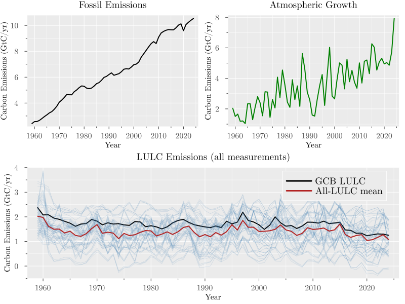
We use annual Global Carbon Budget 2025 data for 1959-2024, with atmospheric growth G_t from NOAA/ESRL global concentration trends¹⁸, fossil emissions excluding carbonation FF_t from the Global Carbon Project fossil dataset¹⁰, and a panel of 69 LULC measurements per year: BLUE¹¹, OSCAR¹², LUCE¹³, and peat-augmented^19–21 process-based land-model combinations drawn from the GCB model ensemble^22–42 (see Methods). The data are shown in Figure 1.

Two LULC means can be constructed from the panel. First, the GCB LULC mean, defined as the mean of the three bookkeeping models (BLUE, OSCAR, and LUCE), corresponds to the LULC column used in the Global Carbon Budget. Second, the all-LULC mean, defined as the cross-series mean across all 69 LULC measurements. The literature has typically used the GCB LULC mean in AF trend estimation, but we show that incorporating the full set of LULC measurements increases the precision of trend estimates and provides more robust inference on trend direction.

To account for the natural variability in the atmospheric growth series^5,7–9, we construct a natural variability adjusted growth series by regressing the observed growth on total anthropogenic emissions (fossil plus LULC) and indices of variability in the El Niño-Southern Oscillation (ENSO) and the Volcanic Aerosol Index (VAI). The fitted values from this regression are used as the natural variability adjusted growth series, which is shown in Figure 1 and used in the main analysis. The details of the regression are described in Methods.

Figure 1: Global Carbon Budget 2025 data for fossil emissions, atmospheric growth, and LULC emissions (1959-2024). For atmospheric growth, we show the observed growth and the natural variability adjusted fit. For the LULC panel, we show all extracted and derived LULC measurements together with the GCB LULC column and the all-LULC cross-series mean.

Identification strategy

The empirical question is whether AF has a positive linear trend. The key design choice is how to use the full panel of repeated LULC measurements while accounting for within-series dependence and cross-series heterogeneity. OLS on a collapsed annual series discards panel information and hence provides less reliable inference, as shown in Table 6 and Table 7. Natural variability in the atmospheric growth series also adds noise to AF estimates, so we use a natural-variability-adjusted growth series in the main analysis to obtain more precise trend estimates. Our preferred specification is a mixed-effects model with random intercepts and random slopes by LULC series, allowing correlation across years within each series and capturing unobserved heterogeneity in LULC measurements^14,15 (see Methods).

For each LULC measurement series, we construct a series of AF estimates by year (Equation 1), and the model estimates a common time trend across all series while allowing for series-specific intercepts and slopes. Formally, the model can be written as AF_{t,j} = \alpha_j + \beta_j t +\varepsilon_{t,j},

where

\alpha_j \sim N(\mu_\alpha, \sigma_\alpha^2),\quad \beta_j \sim N(\mu_\beta, \sigma_\beta^2),\quad \varepsilon_{t,j} \sim N(0, \sigma_\varepsilon^2).

Here \mu_\alpha and \mu_\beta are the fixed effects (overall intercept and slope), while \sigma_\alpha^2 and \sigma_\beta^2 capture the variability in intercepts and slopes across LULC measurement series. The error term \varepsilon_{t,j} captures idiosyncratic noise. The key parameter of interest is \mu_\beta, which captures the average trend across all LULC measurement series. Filtering growth for natural variability and incorporating the full panel of LULC measurements allows us to obtain more precise and robust estimates of the AF trend.

Results

Main estimates

The main results from estimating the mixed-effects model in the full sample are shown in Table 1. The table includes natural-variability-adjusted (AF^{ADJ}) and unadjusted (AF^{RAW}) growth specifications, with and without AR(1) effects in the residuals to control for potential autocorrelation (see Methods).

The slope is positive and statistically significant in all specifications, indicating strong evidence of an increasing AF trend across LULC measurement series. The estimated intercept is around 0.41 and the slope is around 0.0011 per year, implying an increase of about 0.07 in AF over 1959-2024. These estimates are comparable with the approximately 0.45 AF level reported in the literature^2,3,6,7,9,43, while identifying a positive long-run trend when the full LULC-definition ensemble is incorporated. Note that the mixed-effects model reduces uncertainty in the estimates by jointly using this ensemble information, which allows us to obtain more precise estimates and robust inference on trend direction.

Table 1: Mixed-effects model estimates for the full sample (1959-2024). Specifications with natural variability adjusted (ADJ) and unadjusted (RAW) growth rates are shown with and without AR(1) effects.

Mixed-effects model (1959-2024)	AF^{ADJ}	AF^{ADJ} (AR1)	AF^{RAW}	AF^{RAW} (AR1)
Intercept	0.407572	0.408555	0.406959	0.406784
SE (Intercept)	0.005324	0.005546	0.005573	0.005673
p-value (Intercept)	1.0E-5	1.0E-5	1.0E-5	1.0E-5
Slope	0.001082	0.00107	0.001103	0.001117
SE (Slope)	8.6E-5	0.0001	0.000102	0.000108
p-value (Slope)	1.0E-5	1.0E-5	1.0E-5	1.0E-5
AR1		0.177702		0.063011
SE (AR1)		0.031018		0.030731
p-value (AR1)		1.0E-5		0.040326

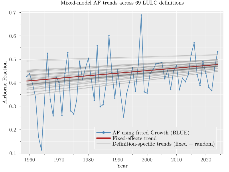
Figure 2 (a) shows the AF series for each LULC measurement together with the overall mixed-effects trend line for the specification using the natural-variability-adjusted growth series and the full sample. The figure shows a clear positive trend across the panel of AF series, with the mixed-effects model capturing this common signal while allowing for series-specific heterogeneity. For visual clarity, one representative AF series is highlighted, while trend lines are estimated using the full LULC-definition ensemble.

(a) AF series with mixed-effects model trend (natural variability adjusted, full sample, 1959-2024).

(b) AF series with mixed-effects model trend (natural variability adjusted, sample ending in 2023).

(c) AF series with WLS trend (natural variability adjusted, full sample, 1959-2024).

(d) AF series with WLS trend (natural variability adjusted, sample ending in 2023).

Figure 2: AF series with mixed-effects and WLS model trends across LULC measurement series.

Endpoint and model specification robustness

AF shows a large value in the final year (2024), so we re-estimate the mixed-effects specification on the sample ending in 2023 to check whether the result is driven by that observation. Results are shown in Table 2 and Figure 2 (b). The slope remains positive and statistically significant, indicating that the increasing AF trend is not driven by the final observation. The slope estimates are smaller, consistent with a contribution from the 2024 large value, but the direction and inference are unchanged.

Table 2: Mixed-effects model estimates for the sample ending in 2023 (1959-2023). Specifications with natural variability adjusted (ADJ) and unadjusted (RAW) growth rates are shown with and without AR(1) effects.

Mixed-effects model (1959-2023)	AF^{ADJ}	AF^{ADJ} (AR1)	AF^{RAW}	AF^{RAW} (AR1)
Intercept	0.409783	0.411223	0.41326	0.413403
SE (Intercept)	0.005345	0.005564	0.005586	0.005677
p-value (Intercept)	1.0E-5	1.0E-5	1.0E-5	1.0E-5
Slope	0.000978	0.000944	0.000808	0.000806
SE (Slope)	8.8E-5	0.000102	0.000103	0.000109
p-value (Slope)	1.0E-5	1.0E-5	1.0E-5	1.0E-5
AR1		0.17795		0.056406
SE (AR1)		0.031115		0.029828
p-value (AR1)		1.0E-5		0.058622

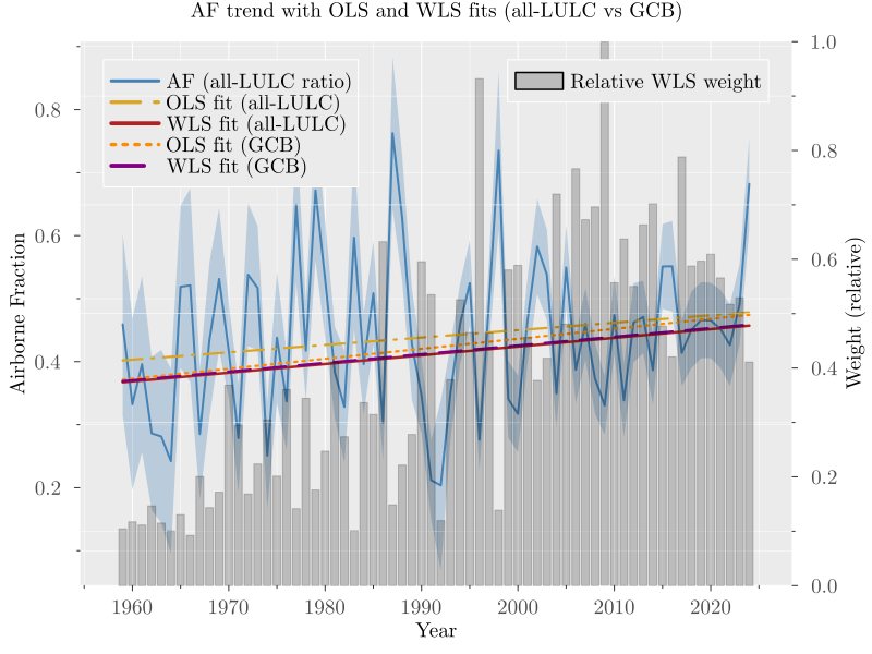
An additional estimation approach that explicitly incorporates denominator measurement uncertainty is WLS estimation of the AF trend, where the weights are constructed from the cross-measurement dispersion of the full LULC panel. Specifically, we estimate a delta-method uncertainty proxy for each annual AF estimate using the cross-measurement dispersion of the full 69-series LULC panel, and use these proxies in a WLS specification^16,17,44 (see Methods). Table 3 reports the results using the all-LULC mean in the denominator estimated by OLS and WLS. The first two columns show the full sample (1959-2024) estimates, while the last two columns show the estimates for the sample ending in 2023 to check whether the results are driven by the large value in 2024. The WLS estimates show a positive and statistically significant slope in both samples, while OLS estimates show a positive but non-significant slope in both samples. Figure 2 (c) and Figure 2 (d) show the WLS trend lines together with the AF series for each LULC measurement for the full sample and the sample ending in 2023, respectively. The WLS trend lines show a clear positive trend across the panel of AF series.

Table 3: Trend comparison for the WLS and OLS estimates with natural variability adjusted growth specifications. The first two columns show the full sample (1959-2024) estimates, while the last two columns show the estimates for the sample ending in 2023.

OLS and WLS	AF^{ADJ} OLS (1959-2024)	AF^{ADJ} WLS (1959-2024)	AF^{ADJ} OLS (1959-2023)	AF^{ADJ} WLS (1959-2023)
Intercept	0.401938	0.367286	0.408212	0.376919
SE (Intercept)	0.029843	0.001243	0.029599	0.001211
p-value (Intercept)	1.0E-5	1.0E-5	1.0E-5	1.0E-5
Slope	0.001172	0.001382	0.000878	0.001054
SE (Slope)	0.000792	2.8E-5	0.000798	2.8E-5
p-value (Slope)	0.138912	1.0E-5	0.271089	1.0E-5

Overall, the results show that incorporating multi-source LULC information and accounting for measurement uncertainty materially changes inference on AF trends. The mixed-effects model, which incorporates the full LULC-definition ensemble and accounts for within-series dependence and cross-series heterogeneity, provides robust evidence of a positive AF trend. The WLS approach, which explicitly incorporates denominator measurement uncertainty, also shows a positive and statistically significant trend.

In contrast, OLS specifications that do not incorporate denominator measurement information provide weaker and less robust evidence, with significance that is sensitive to denominator definition and endpoint exclusion. These results highlight the value of incorporating multi-source LULC information in AF trend estimation in a way that accounts for within-series dependence and cross-series heterogeneity. OLS on a collapsed series discards this information and hence provides less reliable inference on trend direction. Our results clarify why earlier studies that did not incorporate multi-source LULC information have reported weak or inconclusive evidence of an increasing AF trend^1–8.

Additional robustness checks (in Methods), including OLS and WLS specifications in the unadjusted growth series and considering the GCB LULC mean instead of the all-LULC mean, show that the positive AF trend detected by WLS is robust to these alternative specifications, while OLS estimates that do not incorporate multi-source LULC information show weaker evidence of a positive trend and are more sensitive to endpoint exclusion.

Discussion and conclusion

Using a framework that controls for natural variability in the atmospheric growth series and incorporates a broad LULC-definition ensemble from Global Carbon Budget 2025, we find robust evidence that AF increased from 1959 to 2024. Methodologically, incorporating multi-source uncertainty materially changes inference relative to plain OLS. Endpoint tests show that this conclusion is not driven by the large value in 2024.

Our estimates imply that AF increased from about 0.41 around 1960 to about 0.48 by 2024, relative to long-used values around 0.45. For a given emissions pathway, a higher AF would be associated with faster atmospheric CO_2 growth than under a constant-AF baseline, potentially reducing the remaining carbon budget for a given temperature target^1,2,10. Quantifying the budget impact requires dedicated carbon-budget modelling beyond the scope of this study.

References

1.

Canadell, J. G. et al. Contributions to accelerating atmospheric CO_2 growth from economic activity, carbon intensity, and efficiency of natural sinks. Proceedings of the National Academy of Sciences 104, 18866–18870 (2007).

2.

Raupach, M. R. et al. Global and regional drivers of accelerating CO_2 emissions. Proceedings of the National Academy of Sciences 104, 10288–10293 (2007).

3.

Knorr, W. Is the airborne fraction of anthropogenic CO_2 emissions increasing? Geophysical Research Letters 36, L21710 (2009).

4.

Ballantyne, A. P., Alden, C. B., Miller, J. B., Tans, P. P. & White, J. W. C. Increase in observed net carbon dioxide uptake by land and oceans during the past 50 years. Nature 488, 70–72 (2012).

5.

Le Quéré, C. et al. Trends in the sources and sinks of carbon dioxide. Nature Geoscience 2, 831–836 (2009).

6.

Bennedsen, M., Hillebrand, E. & Koopman, S. J. On the evidence of a trend in the CO2 airborne fraction. Nature 616, E1–E3 (2023).

7.

Bennedsen, M., Hillebrand, E. & Koopman, S. J. A regression-based approach to the CO2 airborne fraction. Nature Communications 15, 8507 (2024).

8.

Bennett, B. F., Salawitch, R. J., McBride, L. A., Hope, A. P. & Tribett, W. R. Quantification of the Airborne Fraction of Atmospheric CO_{\textrm{2}} Reveals Stability in Global Carbon Sinks Over the Past Six Decades. Journal of Geophysical Research: Biogeosciences 129, e2023JG007760 (2024).

9.

Vera-Valdés, J. E. & Grivas, C. Robust estimation of carbon dioxide airborne fraction under measurement errors. Environmental Research Communications 7, 031009 (2025).

10.

Friedlingstein, P. et al. Global carbon budget 2025. Earth System Science Data 18, 3211–3288 (2026).

11.

Hansis, E., Davis, S. J. & Pongratz, J. Relevance of methodological choices for accounting of land use change carbon fluxes. Global Biogeochemical Cycles 29, 1230–1246 (2015).

12.

Gasser, T. et al. Historical CO2 emissions from land use and land cover change and their uncertainty. Biogeosciences 17, 4075–4101 (2020).

13.

Qin, Z. et al. Global spatially explicit carbon emissions from land-use change over the past six decades (1961-2020). One Earth 7, 835–847 (2024).

14.

Henderson, C. R. Estimation of variance and covariance components. Biometrics 9, 226–252 (1953).

15.

Bolker, B. M. et al. Generalized linear mixed models: A practical guide for ecology and evolution. Trends in Ecology & Evolution 24, 127–135 (2009).

16.

Fuller, W. A. Measurement Error Models. (Wiley, New York, 1987).

17.

Carroll, R. J., Ruppert, D., Stefanski, L. A. & Crainiceanu, C. M. Measurement Error in Nonlinear Models: A Modern Perspective. (Chapman & Hall/CRC, Boca Raton, 2006).

18.

Lan, X., Tans, P. & Thoning, K. W. Trends in globally-averaged CO2 determined from NOAA global monitoring laboratory measurements. (2026) doi:10.15138/9N0H-ZH07.

19.

Conchedda, G. & Tubiello, F. N. Drainage of organic soils and GHG emissions: Validation with country data. Earth System Science Data 12, 3113–3137 (2020).

20.

Müller, J. & Joos, F. Committed and projected future changes in global peatlands – continued transient model simulations since the last glacial maximum. Biogeosciences 18, 3657–3687 (2021).

21.

Qiu, C. et al. Large historical carbon emissions from cultivated northern peatlands. Science Advances 7, eabf1332 (2021).

22.

Haverd, V. et al. A new version of the CABLE land surface model (subversion revision r4601) incorporating land use and land cover change, woody vegetation demography, and a novel optimisation-based approach to plant coordination of photosynthesis. Geoscientific Model Development 11, 2995–3026 (2018).

23.

Melton, J. R. et al. CLASSIC v1.0: The open-source community successor to the canadian land surface scheme (CLASS) and the canadian terrestrial ecosystem model (CTEM) – part 1: Model framework and site-level performance. Geoscientific Model Development 13, 2825–2850 (2020).

24.

Lawrence, D. M. et al. The community land model version 5: Description of new features, benchmarking, and impact of forcing uncertainty. Journal of Advances in Modeling Earth Systems 11, 4245–4287 (2019).

25.

Fisher, R. A. et al. Taking off the training wheels: The properties of a dynamic vegetation model without climate envelopes, CLM4.5(ED). Geoscientific Model Development 8, 3593–3619 (2015).

26.

Tian, H. et al. North american terrestrial CO2 uptake largely offset by CH4 and N2O emissions: Toward a full accounting of the greenhouse gas budget. Climatic Change 129, 423–426 (2015).

27.

Ma, L. et al. Global evaluation of the ecosystem demography model (ED v3.0). Geoscientific Model Development 15, 1971–1994 (2022).

28.

Yang, X., Thornton, P., Ricciuto, D., Wang, Y. & Hoffman, F. Global evaluation of terrestrial biogeochemistry in the energy exascale earth system model (E3SM) and the role of the phosphorus cycle in the historical terrestrial carbon balance. Biogeosciences 20, 2813–2836 (2023).

29.

Needham, J. et al. Vertical canopy gradients of respiration drive plant carbon budgets and leaf area index. New Phytologist 246, 144–157 (2025).

30.

Felzer, B. S. & Jiang, M. Effect of land use and land cover change in context of growth enhancements in the united states since 1700: Net source or sink? Journal of Geophysical Research: Biogeosciences 123, 3439–3457 (2018).

31.

Xia, J. Z. et al. The carbon budget of china: 1980–2021. Science Bulletin 69, 114–124 (2024).

32.

Yue, X. et al. Development and evaluation of the interactive model for air pollution and land ecosystems (iMAPLE) version 1.0. Geoscientific Model Development 17, 4621–4642 (2024).

33.

Shu, S., Jain, A. K., Koven, C. D. & Mishra, U. Estimation of permafrost SOC stock and turnover time using a land surface model with vertical heterogeneity of permafrost soils. Global Biogeochemical Cycles 34, e2020GB006585 (2020).

34.

Reick, C. H. et al. JSBACH 3 - the land component of the MPI earth system model: Documentation of version 3.2. (2021) doi:10.17617/2.3279802.

35.

Poulter, B., Frank, D. C., Hodson, E. L. & Zimmermann, N. E. Impacts of land cover and climate data selection on understanding terrestrial carbon dynamics and the CO2 airborne fraction. Biogeosciences 8, 2027–2036 (2011).

36.

Smith, B. et al. Implications of incorporating n cycling and n limitations on primary production in an individual-based dynamic vegetation model. Biogeosciences 11, 2027–2054 (2014).

37.

Schaphoff, S. et al. LPJmL4 – a dynamic global vegetation model with managed land – part 1: Model description. Geoscientific Model Development 11, 1343–1375 (2018).

38.

Lienert, S. & Joos, F. A bayesian ensemble data assimilation to constrain model parameters and land-use carbon emissions. Biogeosciences 15, 2909–2930 (2018).

39.

Vuichard, N. et al. Accounting for carbon and nitrogen interactions in the global terrestrial ecosystem model ORCHIDEE (trunk version, rev 4999): Multi-scale evaluation of gross primary production. Geoscientific Model Development 12, 4751–4779 (2019).

40.

Walker, A. P. et al. The impact of alternative trait-scaling hypotheses for the maximum photosynthetic carboxylation rate (v-cmax) on global gross primary production. New Phytologist 215, 1370–1386 (2017).

41.

Kato, E., Kinoshita, T., Ito, A., Kawamiya, M. & Yamagata, Y. Evaluation of spatially explicit emission scenario of land-use change and biomass burning using a process-based biogeochemical model. Journal of Land Use Science 8, 104–122 (2013).

42.

Ito, A. Disequilibrium of terrestrial ecosystem CO2 budget caused by disturbance-induced emissions and non-CO2 carbon export flows: A global model assessment. Earth System Dynamics 10, 685–709 (2019).

43.

Gloor, M. et al. What can be learned about carbon cycle climate feedbacks from the CO2 airborne fraction? Atmospheric Chemistry and Physics 10, 7739–7752 (2010).

44.

Oehlert, G. W. A note on the delta method. The American Statistician 46, 27–29 (1992).

45.

Aitken, A. C. On least squares and linear combination of observations. Proceedings of the Royal Society of Edinburgh 55, 42–48 (1935).

46.

Huang, B. et al. Extended reconstructed sea surface temperature, version 5 (ERSSTv5): Upgrades, validations, and intercomparisons. Journal of Climate https://doi.org/10.1175/JCLI-D-16-0836.1 (2017) doi:10.1175/JCLI-D-16-0836.1.

47.

Ammann, C. M., Meehl, G. A., Washington, W. M. & Zender, C. S. A monthly and latitudinally varying volcanic forcing dataset in simulations of 20th century climate. Geophysical Research Letters 30, (2003).

Methods

Our primary estimator is a linear mixed-effects trend model with random intercepts and random slopes for each LULC measurement series^14,15. As a robustness check, we also estimate a measurement-error-aware airborne fraction variance using repeated yearly denominator measurements, followed by WLS trend estimation^16,17,44,45.

Construction of the LULC measurement panel

The repeated LULC measurements are built from the Global Carbon Budget 2025 dataset. We first extract the three bookkeeping series: BLUE¹¹, OSCAR¹², LUCE¹³. Then, for each process-based land-model LULC series in the GCB ensemble that does not already include peat emissions^22–42, we add one peat component measurement to make it comparable to the bookkeeping models, which include peat emissions by construction. Specifically, for each of the 22 process-based series we create 3 peat-augmented variants by adding FAO_peat, LPX_Bern_peat, and ORCHIDEE_peat^19–21, respectively. This produces 66 derived series, and together with BLUE/OSCAR/LUCE gives a panel of 69 yearly LULC measurements.

Accounting for natural variability

Natural factors such as volcanic eruptions and El Niño events can cause year-to-year fluctuations in atmospheric CO_2 growth that are not directly related to anthropogenic emissions. To account for this natural variability, we consider a specification that includes a control for the Niño 3 index, which captures El Niño–Southern Oscillation (ENSO) variability and Volcanic Aerosol Index (VAI) to capture volcanic activity.

The specification is as follows: \hat{G}_t = \gamma_0 + \gamma_1 \hat{C}_t + \gamma_2 \text{N3}_t + \gamma_3 \text{VAI}_t + \varepsilon_{t,j}, \tag{2}

where \hat{C}_t is the estimated total emissions (fossil fuel plus LULC), \text{N3}_t is the Niño 3 index, and \text{VAI}_t is the Volcanic Aerosol Index for year t. The error term captures idiosyncratic noise.

In the estimation, the yearly total emissions (\hat{C}_t) are computed as the sum of fossil fuel emissions and the mean of the LULC panel for that year as \hat C_t = FF_t + \bar{LULC}_t, \qquad \bar{LULC}_t = \frac{1}{n_t}\sum_{j=1}^{n_t} LULC_{tj},

where n_t=3 for the GCB LULC mean and n_t=69 for the all-LULC mean.

To account for uncertainty in the LULC measurements, we use WLS in Equation 2 with weights based on the cross-measurement empirical dispersion of the full LULC panel

\widehat{\operatorname{Var}}({\hat{C}_t}) = \frac{1}{n_t-1} \sum_{j=1}^{n_t} (C_{tj} - \hat{C}_t)^2,

where C_{tj} = FF_t + LULC_{tj} is the total emissions for year t using the j-th LULC measurement and n_t=69 is the number of LULC measurements. This weighting scheme gives less weight to years with higher cross-measurement dispersion or more uncertainty in the total emissions estimate.

The variance of \hat{G}_t is estimated using the delta method, which accounts for the uncertainty in the regression coefficients and the variability in the LULC measurements. For the linear model specified above, the variance of the fitted values \hat{G}_t can be approximated using the delta method as

\widehat{\operatorname{Var}}(\hat{G}_t) = \gamma_1^2 \operatorname{\widehat{Var}}(\hat{C}_t).

The weights used in the WLS regression are hence given by w_t = \frac{1}{\gamma_1^2 \operatorname{\widehat{Var}}(\hat{C}_t)}, which reflects the uncertainty in the fitted values due to the variability in the LULC measurements.

Results from the growth regression estimated by WLS are shown in Table 4.

Table 4: Growth regression with natural variability controls.

Growth equation	Estimate	Std. error	p-value
Intercept	1.071015	0.340529	0.001660
Total emissions	0.364301	0.038410	1.0E-5
VAI	-17.386855	3.081315	1.0E-5
N3 index	1.054167	0.131682	1.0E-5
R-squared	0.831525

The fitted values \hat{G}_t represent the natural variability adjusted growth series, which is shown in Figure 1 and used in the main analysis. The variance of the fitted values, which captures the uncertainty in the growth estimates due to variability in the LULC measurements, is used to construct weights for the WLS regression on AF trends as described below.

Mixed-effects model

The primary estimator is a linear mixed-effects trend model fitted on the panel of yearly AF values constructed from each LULC measurement series. For each year t and series j, we define

AF_{t,j} = \frac{\hat{G}_t}{FF_t + LULC_{t,j}},

where \hat{G}_t is the fitted value from the growth regression that accounts for natural variability, FF_t is fossil fuel emissions, and LULC_{t,j} is the j-th LULC measurement for year t. We then fit a mixed-effects model to these AF estimates, allowing for random intercepts and slopes by LULC series, to capture heterogeneity across series and estimate

AF_{t,j} = (\mu_\alpha + u_{\alpha j}) + (\mu_\beta + u_{\beta j})\,t + \varepsilon_{t,j},

with

\begin{bmatrix}u_{\alpha j} \\ u_{\beta j}\end{bmatrix} \sim N\!\left( \begin{bmatrix}0\\0\end{bmatrix}, \Sigma_u \right), \qquad \varepsilon_{t,j} \sim N(0,\sigma_\varepsilon^2).

This specification allows each LULC series to have its own level and trend while estimating a common population-average trend \mu_\beta. The main estimand is \mu_\beta, interpreted as the average annual change in AF across the full set of LULC definitions. Note that this notation is equivalent to the more compact notation in the main text, where \alpha_j = \mu_\alpha + u_{\alpha j} and \beta_j = \mu_\beta + u_{\beta j}.

The model is estimated by restricted maximum likelihood^14,15. Fixed-effect uncertainty is based on model-based standard errors and Wald tests. We report the estimated fixed intercept and slope, standard errors, and p-values.

Identification and interpretation rely on standard mixed-model conditions: (i) conditional linearity in time, (ii) random effects centred at zero and independent across LULC definitions, and (iii) mean-zero residuals conditional on fixed and random effects.

Robustness exercises for the mixed-effects model

To control for potential autocorrelation in the residuals, we consider a specification that includes an AR(1) structure on \varepsilon_{t,j}:

\varepsilon_{t,j} = \rho \varepsilon_{t-1,j} + \eta_{t,j}, \quad \eta_{t,j} \sim N(0,\sigma_\eta^2).

This specification is estimated on the full sample and the sample ending in 2023, considering both the natural variability adjusted and unadjusted growth series.

Weighted least squares estimation approach

As an alternative estimation approach that explicitly incorporates denominator measurement uncertainty and serves as a robustness exercise to the mixed-effects model, we also estimate a two-stage measurement-error-aware WLS model that uses repeated LULC measurements to construct a denominator-uncertainty proxy for each year^16,17,44,45.

Assume for each time t=1,\dots,T we observe:

• atmospheric growth adjusted for natural variability, \hat{G}_t, together with its variance as estimated above, \operatorname{Var}(\hat{G}_t), and

• multiple denominator measurements c_{t1},\dots,c_{t n_t} with n_t \ge 2, which are noisy observations of a latent C_t.

Using all denominator measurements, we construct a year-specific uncertainty proxy for the ratio estimator AF_t = \hat{G}_t/C_t via the delta method, which captures how dispersion in both numerator and denominator definitions propagates into AF. The procedure is described in detail next.

Delta method for ratio variance estimation

Define the random vector and the function of interest as X_t= \begin{bmatrix} \hat{G}_t\\ \hat C_t \end{bmatrix}, \qquad g(X_t)=\frac{\hat{G}_t}{\hat C_t}.

and let \sigma_{G,t}^2 = \operatorname{Var}(\hat{G}_t),\qquad \sigma_{C,t}^2 = \operatorname{Var}(\hat C_t),\qquad \sigma_{GC,t} = \operatorname{Cov}(\hat{G}_t,\hat C_t).

1. Linearize g around the mean vector (\mu_{G,t},\mu_{C,t})=\mathbb E[(\hat{G}_t,\hat C_t)]: g(X_t)\approx g(\mu_{G,t},\mu_{C,t})+\nabla g(\mu_{G,t},\mu_{C,t})^\top (X_t-\mathbb E[X_t]).

2. Compute the gradient: \nabla g(G,C)= \begin{bmatrix} \partial g/\partial G\\ \partial g/\partial C \end{bmatrix} = \begin{bmatrix} 1/C\\ -G/C^2 \end{bmatrix}.

3. Write the covariance matrix of (\hat{G}_t,\hat C_t): \Sigma_t= \begin{bmatrix} \sigma_{G,t}^2 & \sigma_{GC,t}\\ \sigma_{GC,t} & \sigma_{C,t}^2 \end{bmatrix}.

4. Apply the delta-method variance formula \operatorname{Var}(g(X_t))\approx \nabla g(\mu_{G,t},\mu_{C,t})^\top\Sigma_t\nabla g(\mu_{G,t},\mu_{C,t}), and with plug-in evaluation at (G_t,C_t), this becomes

\operatorname{Var}(AF_t)\approx\left(\frac{1}{C_t}\right)^2 \sigma_{G,t}^2+\left(\frac{G_t}{C_t^2}\right)^2 \sigma_{C,t}^2-2\frac{G_t}{C_t^3}\sigma_{GC,t}.

In practice, we use plug-in estimates (replace unknown moments by their empirical counterparts):

\sigma^2_{G,t} \approx \widehat{\operatorname{Var}}(\hat{G}_t),\qquad \sigma^2_{C,t} \approx \widehat{\operatorname{Var}}(\hat C_t),\qquad \sigma_{GC,t} \approx 0,

where we set the covariance term to zero to guarantee that the variance estimate is always positive.

This yields the following variance proxy for AF_t:

\widehat{\operatorname{Var}}(AF_t) = \left(\frac{1}{C_t}\right)^2 \widehat{\operatorname{Var}}(\hat{G}_t) + \left(\frac{G_t}{C_t^2}\right)^2 \widehat{\operatorname{Var}}(\hat C_t).

WLS regression of AF_t on time

For each time t, we obtain a point estimate AF_t and an uncertainty proxy that reflects cross-measurement dispersion. We use these quantities to fit a linear trend via WLS:

AF_t = \alpha + \beta t + \varepsilon_t, \quad \varepsilon_t \sim (0, \sigma_t^2), \quad \sigma_t^2 = \operatorname{Var}(AF_t).

In our application, the weighting term, w_t=\frac{1}{\sigma_t^2}, is obtained from AF uncertainty from denominator dispersion and varies across years with the spread of the LULC measurement panel. We use this term to weight the regression, giving more weight to years with lower denominator-related uncertainty. The core idea is that years with more consistent LULC measurements provide more reliable AF estimates, and hence should have greater influence on the trend estimation.

Testing for a time trend is then a test of \beta=0 versus \beta\neq 0 in this linear model, and WLS uses the repeated denominator information through this delta-method weighting scheme.

Robustness exercises for the WLS model

As robustness checks, we consider alternative specifications of the WLS model. First, we consider a specification using the unadjusted observed growth G_t instead of the natural variability adjusted growth \hat{G}_t to check whether the results are sensitive to the choice of growth series, and the results, shown in Table 5, remain qualitatively similar.

Table 5: Trend comparison for the WLS and OLS estimates on the full sample (1959-2023), with natural variability adjusted and unadjusted growth specifications.

OLS and WLS	AF^{RAW} OLS (1959-2024)	AF^{RAW} WLS (1959-2024)	AF^{RAW} OLS (1959-2023)	AF^{RAW} WLS (1959-2023)
Intercept	0.40194	0.30194	0.40821	0.30982
SE (Intercept)	0.02984	0.00095	0.0296	0.00093
p-value (Intercept)	1.0E-5	1.0E-5	1.0E-5	1.0E-5
Slope	0.00117	0.0023	0.00088	0.00202
SE (Slope)	0.00079	2.0E-5	0.0008	2.0E-5
p-value (Slope)	0.13891	1.0E-5	0.27109	1.0E-5

Then, we consider a specification using the GCB LULC mean instead of the all-LULC mean in the denominator to check whether the results are sensitive to the choice of denominator definition. The results remain robust, showing a positive and statistically significant trend in AF on both the full sample, Table 6, and the sample ending in 2023, Table 7.

Table 6: Trend comparison for the GCB mean, full sample, with adjusted and unadjusted growth specifications.

OLS and WLS (1959-2024) GCB mean	AF^{ADJ} (OLS)	AF^{ADJ} (WLS)	AF^{RAW} (OLS)	AF^{RAW} (WLS)
Intercept	0.371410	0.368874	0.377502	0.392029
SE (Intercept)	0.029039	0.000777	0.028805	0.000474
p-value (Intercept)	1.0E-5	1.0E-5	1.0E-5	1.0E-5
Slope	0.001581	0.001382	0.001580	0.002650
SE (Slope)	0.000771	1.7E-5	0.000770	2.0E-5
p-value (Slope)	0.040212	1.0E-5	0.040210	1.0E-5

Table 7: Trend comparison for the GCB mean, sample ending in 2023, with adjusted and unadjusted growth specifications.

OLS and WLS (1959-2023) GCB mean	AF^{ADJ} (OLS)	AF^{ADJ} (WLS)	AF^{RAW} (OLS)	AF^{RAW} (WLS)
Intercept	0.377502	0.380109	0.377500	0.283400
SE (Intercept)	0.028805	0.000758	0.028810	0.000910
p-value (Intercept)	1.0E-5	1.0E-5	1.0E-5	1.0E-5
Slope	0.001296	0.001030	0.001300	0.002370
SE (Slope)	0.000777	1.7E-5	0.000780	2.0E-5
p-value (Slope)	0.095163	1.0E-5	0.095160	1.0E-5

OLS specification

As a point of comparison, we also estimate a simple OLS specification that regresses AF on time using a single denominator definition (either the GCB LULC mean or the all-LULC mean) without incorporating the multi-source LULC information. This specification is estimated for both the full sample and the sample ending in 2023, and considering the natural variability adjusted growth series and the unadjusted growth series. The OLS results show weaker evidence of a positive trend and greater sensitivity to endpoint exclusion compared to the mixed-effects and WLS specifications, highlighting the value of incorporating multi-source LULC information in AF trend estimation.

Data availability

The study uses publicly available Global Carbon Budget 2025 data. The GCB data can be accessed at https://globalcarbonbudget.org/gcb-2025/. To control for natural variability, we use publicly available Niño 3 index data and Volcanic Aerosol Index data. The Niño 3 index data⁴⁶ was obtained from the NOAA Physical Sciences Laboratory, available at https://psl.noaa.gov/data/timeseries/monthly/NINO3/, and the Volcanic Aerosol Index data⁴⁷ from the NOAA National Centers for Environmental Information, available at https://www.ncei.noaa.gov/access/paleo-search/study/5786. All data used in the analysis, including the extracted and derived LULC panel, are available in the manuscript repository at github.com/everval/Airborne-Fraction-WLS-Trend.

Code availability

All code used to process data, estimate models, and generate figures is available in the manuscript repository (github.com/everval/Airborne-Fraction-WLS-Trend) inside the scripts folder, including Quarto analysis files and Julia and R helper functions. The processed analysis tables are provided inside the results folder. The code is licensed under the MIT License, and the repository includes a README file with instructions for reproducing the analysis.

Preprint availability

A preprint of this manuscript is available on arXiv (2605.30242).

Competing interests

The author declares no competing interests.