Global Temperature Anomalies in Practice

An Open, Reproducible Framework for Baseline Harmonisation and ENSO-Aware Visualisation

Author

Affiliations

Aalborg University

CoRE

Abstract

We present a reproducible pipeline for downloading, processing, and harmonising global temperature anomaly series from HadCRUT5, GISTEMP, NOAAGlobalTemp, Berkeley Earth, and ERA5. All datasets are aligned to a common 1850-1900 pre-industrial baseline to enable direct comparison. The workflow also integrates the Oceanic Niño Index (ONI) to annotate El Niño and La Niña phases in the figures, helping distinguish short-term variability from the long-term warming signal. Final outputs are exported as transparent, analysis-ready CSV files, available through the repository.

Keywords

Global Temperature Anomalies, Pre-industrial Baseline, El Niño Southern Oscillation

Introduction

Global temperature anomalies are central to climate variability and change analysis, but practical use across datasets is often limited by inconsistent baseline periods and heterogeneous data formats. Table 1 summarises the baseline periods, formats, and key notes for five of the most widely used global temperature anomaly datasets.

Table 1: Baseline periods and processing considerations for major global temperature anomaly datasets.¹

Dataset	Baseline period	Format	Practical note
HadCRUT5(Morice et al. 2021)	1961–1990	CSV	Release lag is typically longer than for the other datasets.
NOAAGlobalTemp(Huang et al. 2024)	1991–2020	ASCII	Data is presented using space-delimited files. File names are versioned, so the download URL changes over time.
GISTEMP(GISTEMP 2020)	1951–1980	CSV	Series begins in 1880, so an additional pre-industrial adjustment is needed. Data is in wide format.
Berkeley Earth(Rohde and Hausfather 2020)	1951–1980	TXT	Distributed as space-delimited text files.
ERA5(Hersbach et al. 2023)	No fixed baseline	NetCDF	No global average anomaly is provided; users must compute anomalies relative to a selected climatology. Requires setting up a key for accessing the data.

The table highlights two recurring operational barriers: heterogeneous file structures and inconsistent baseline definitions. Together, these barriers reduce comparability, increase processing overhead, and weaken reproducibility in applied climate analysis.

This paper addresses these barriers with a concise, reusable workflow that harmonises all series to a common 1850-1900 reference and a shared tabular format. The implementation is written in Julia (Bezanson et al. 2017) for clarity, speed, and straightforward reproducibility.

We standardise all datasets listed in Table 1, compute anomalies relative to the common baseline, and produce a unified analysis table. To support interpretation, we integrate the Oceanic Niño Index (Huang et al. 2025a, 2025b; NOAA National Centers for Environmental Information 2026) and annotate El Niño and La Niña phases in the plots, separating short-term ENSO variability from long-run warming.

The remainder of the paper proceeds from environment setup and source-specific processing to dataset merging and comparative visualisation with ENSO overlays.

Necessary Packages and Helper Functions

This notebook uses a Julia project environment with pinned dependencies. The workflow makes use of several packages for data download, processing, and visualisation: CDSAPI (Chan and contributors 2026), CSV (Quinn and contributors 2026), Dates, DataFrames (Bouchet-Valat and Kamiński 2023), HTTP (JuliaWeb contributors 2026), NCDatasets (Barth 2024), Plots (Christ et al. 2023), and Statistics.

Dates and Statistics are included in the Julia standard library; the remaining packages can be installed with Pkg.add. The code snippet below shows how to add the necessary packages. This step only needs to be done once, and the resulting Project.toml and Manifest.toml files will capture the exact versions used for reproducibility.

Pkg.add(["CDSAPI", "CSV", "DataFrames", "HTTP", "NCDatasets", "Plots"])

After installation, packages are loaded with using.

using CDSAPI, CSV, DataFrames, Dates, HTTP, NCDatasets, Plots, Statistics

Each dataset follows four steps: (1) download, (2) standardise to date–anomaly format, (3) adjust to 1850–1900 baseline, (4) save as CSV. Helper functions below support this workflow.

A utility function streamlines baseline calculations:

function adjust_baseline(df, temp_col; start_year=1850, end_year=1900, date_col=:Date)
    """Compute baseline mean and adjust temperature anomalies."""
    oldbase = mean(df[(df[!, date_col].>=Date(start_year, 1, 1)).&(df[!, date_col].<Date(end_year, 1, 1)), temp_col])
    return df[!, temp_col] .- oldbase
end

HadCRUT5

The HadCRUT5 dataset is provided by the Met Office Hadley Centre and the Climatic Research Unit at the University of East Anglia (Morice et al. 2021). The HadCRUT5 dataset is available in CSV format from the Met Office website.

hfilename = "data/HadCRUT5_global_monthly_average.csv"
open(hfilename, "w") do io
    write(io, HTTP.get("https://www.metoffice.gov.uk/hadobs/hadcrut5/data/HadCRUT.5.1.0.0/analysis/diagnostics/HadCRUT.5.1.0.0.analysis.summary_series.global.monthly.csv").body)
end
rawhadcrut = CSV.read(hfilename, DataFrame)
rename!(rawhadcrut, :Time => :Date, :"Anomaly (deg C)" => :RawTemperature)
hadcrut = rawhadcrut[!, [:Date, :RawTemperature]]
hadcrut[!, :Temp] = adjust_baseline(hadcrut, :RawTemperature)
CSV.write(hfilename, hadcrut)

NOAAGlobalTemp

The NOAAGlobalTemp dataset is provided by the National Oceanic and Atmospheric Administration (NOAA) (Huang et al. 2024). It is available in ASCII format from the NOAA NCEI website, where space-delimited files are used. The URL of the dataset depends on the month of the data; note the ...YYYYMM.asc name in the URL.

nfilename = "data/NOAA_global_monthly_average.csv"
open(nfilename, "w") do io
    write(io, HTTP.get("https://www.ncei.noaa.gov/data/noaa-global-surface-temperature/v6.1/access/timeseries/aravg.mon.land_ocean.90S.90N.v6.1.0.202603.asc").body)
end
# Convert space-delimited ASCII to CSV
write(nfilename, join([join(split(strip(line)), ",") for line in readlines(nfilename)], "\n"))
rawnoaa = CSV.read(nfilename, DataFrame; delim=',', header=0)
dates = Date.(rawnoaa.Column1, rawnoaa.Column2, 1)
noaa = DataFrame(:Date=>dates, :RawTemp=>rawnoaa.Column3)
noaa[!, :Temp] = adjust_baseline(noaa, :RawTemp)
CSV.write(nfilename, noaa)

GISTEMP

The GISTEMP dataset (GISTEMP 2020) is available in CSV format from the NASA GISS website. The data is provided in a wide format, where each row corresponds to one year and monthly values are stored in separate columns. To process this data, we need to convert it to a long format, where each row corresponds to a single month. The longseries function defined below performs this conversion.

function longseries(data)
    """Convert wide-format (year rows) to long-format (monthly rows)."""
    height, last_row = size(data, 1), 12 - count(ismissing, data[end, 2:13])
    many, long = (height - 1) * 12 + last_row, zeros(many, 1)
    for ii in 1:(height-1), jj in 1:12
        long[(ii-1)*12+jj] = data[ii, jj+1]
    end
    for jj in 1:last_row
        long[(height-1)*12+jj] = data[height, jj+1]
    end
    return long
end

The function takes a DataFrame in wide format and returns a long-format array. It calculates the total number of months based on the number of years, same as the number of rows, and the number of non-missing months in the last year. It then fills the long-format array by looping through the years and months.

Once the longseries function is defined, we can use it to process the GISTEMP data. Note that the data is cleaned from the *** string used to denote missing values. Furthermore, a date array is created based on the number of months in the dataset, starting from January 1880. The raw temperature anomalies are then adjusted to calculate anomalies relative to the 1850-1900 baseline. Following the data source recommendation, the data are first adjusted to an 1880-1900 baseline and then shifted by 0.038°C to account for pre-1880 conditions².

gfilename = "data/GISTEMP_global_monthly_average.csv"
open(gfilename, "w") do io
    write(io, HTTP.get("https://data.giss.nasa.gov/gistemp/tabledata_v4/GLB.Ts%2BdSST.csv").body)
end
longgistemp = CSV.read(gfilename, DataFrame, header=2, missingstring=["***"])
gistemp_long = longseries(longgistemp)[:]
Tt = length(gistemp_long) - 1
dates = collect(Date(1880, 1, 1):Month(1):Date(1880, 1, 1) + Month(Tt))
gistemp = DataFrame(:Date=>dates, :RawTemp=>gistemp_long)
gistemp[!, :Temp] = adjust_baseline(gistemp, :RawTemp, start_year=1880) .+ 0.038  # +0.038°C pre-1880 offset per GISS
CSV.write(gfilename, gistemp)

Berkeley Earth

The Berkeley Earth dataset (Rohde and Hausfather 2020) is available in TXT format from the Berkeley Earth website using space-delimited files.

bfilename = "data/BerkeleyEarth_global_monthly_average.csv"
open(bfilename, "w") do io
    write(io, HTTP.get("https://storage.googleapis.com/berkeley-earth-temperature-hr/global/Global_TAVG_monthly.txt").body)
end
rawtemp = CSV.read(bfilename, DataFrame, comment="%", delim=" ", ignorerepeated=true)
rename!(rawtemp, [:Year, :Month, :Anomaly_Monthly, :Unc_Monthly, :Anomaly_Annual,
 :Unc_Annual, :Anomaly_5yr, :Unc_5yr, :Anomaly_10yr, :Unc_10yr, :Anomaly_20yr, :Unc_20yr])
rawtemp.Date = Date.(rawtemp.Year, rawtemp.Month, 1)
rawtemp.Temp = adjust_baseline(rawtemp, :Anomaly_Monthly)
berkeley = rawtemp[!, [:Date, :Anomaly_Monthly, :Temp]]
rename!(berkeley, :Anomaly_Monthly => :RawTemperature)
CSV.write(bfilename, berkeley)

Note that a new variable is created to store the date, which is constructed from the year and month columns in the dataset.

ERA5

ERA5 is the fifth generation ECMWF reanalysis for the global climate and weather (Hersbach et al. 2023). Data is available from 1940 in NetCDF format from the Copernicus Climate Data Store.

The API requires setting up a personal key in a .cdsapirc file, which should be placed in the root directory of the project. You can get a key by requesting it at the Copernicus Climate Data Store website. The code below assumes that you have already set up the .cdsapirc file with your key. To obtain the full dataset, the whole period from 1940 to 2026 is requested, but the file is large, close to 1.5 GB. For update purposes, the code can be modified to request a smaller period, for example, from 2020 to present. The code also specifies the variable to download (2m temperature), the time resolution (monthly), and the data format (NetCDF).

# Download ERA5 and compute global mean by month
dataset = "reanalysis-era5-single-levels-monthly-means"
request = """{"product_type": ["monthly_averaged_reanalysis"], "variable": ["2m_temperature"],
    "year": ["1940", "1941", "1942", "1943", "1944", "1945", "1946", "1947", "1948", "1949", 
        "1950", "1951", "1952", "1953", "1954", "1955", "1956", "1957", "1958", "1959",
        "1960", "1961", "1962", "1963", "1964", "1965", "1966", "1967", "1968", "1969",
        "1970", "1971", "1972", "1973", "1974", "1975", "1976", "1977", "1978", "1979",
        "1980", "1981", "1982", "1983", "1984", "1985", "1986", "1987", "1988", "1989",
        "1990", "1991", "1992", "1993", "1994", "1995", "1996", "1997", "1998", "1999",
        "2000", "2001", "2002", "2003", "2004", "2005", "2006", "2007", "2008", "2009",
        "2010", "2011", "2012", "2013", "2014", "2015", "2016", "2017", "2018", "2019",
        "2020", "2021", "2022", "2023", "2024", "2025", "2026"],
    "month": ["01", "02", "03", "04", "05", "06", "07", "08", "09", "10", "11", "12"],
    "time": ["00:00"], "data_format": "netcdf", "download_format": "unarchived"}"""
CDSAPI.retrieve(dataset, request, "data/era5_2m_temperature.nc")

The next code snippet computes monthly global mean temperature from gridded ERA5 data. Latitude weights are based on the cosine of latitude to account for grid-cell area differences, so high-latitude cells receive less weight than equatorial cells. ERA5 values are reported in Kelvin and are converted to degrees Celsius.

filename = "data/era5_2m_temperature.nc"
ds = NCDataset(filename, "r")
lat_era = ds["latitude"][:]
time_era = ds["valid_time"][:]
date_era = Date.(time_era)

global_mean_C = zeros(length(date_era))
weights = cos.(lat_era * π / 180)
for i in 1:length(date_era)
    t2m = ds["t2m"][:, :, i]  # [lon, lat] in K
    global_mean_K = sum(mean(t2m, dims=1)' .* weights) / sum(weights)
    global_mean_C[i] = global_mean_K - 273.15
end

Once the monthly global mean temperatures are calculated, anomalies can be computed relative to the 1850-1900 baseline. Unlike the other datasets, ERA5 does not provide a fixed baseline period, so we first compute monthly climatology over 1991-2020 and then derive anomalies relative to that reference. Finally, we add an offset to approximate pre-industrial anomalies and save the processed data.³

time_dates = date_era
start_1991 = findfirst(≥(Date(1991,1,1)), time_dates)
end_2020 = findfirst(≥(Date(2021,1,1)), time_dates) - 1
month_clim = [mean(global_mean_C[start_1991:end_2020]
[month.(time_dates[start_1991:end_2020]).==m]) for m in 1:12]
anom_1991_2020 = global_mean_C .- month_clim[month.(time_dates)]
pa_anom = anom_1991_2020 .+ 0.88  # Pre-industrial offset
era5 = DataFrame(Date=time_dates, RawTemperature=anom_1991_2020, Temp=pa_anom)
CSV.write("data/ERA5_global_monthly_average.csv", era5)

Oceanic Niño Index (ONI)

El Niño (La Niña) is defined as the 3-month running mean of sea surface temperature anomalies in Niño 3.4 region exceeding +0.5°C (or below −0.5°C) for five consecutive overlapping seasons. The data is obtained from the Extended Reconstructed Sea Surface Temperature (ERSST) dataset, which is a global monthly analysis of sea surface temperature data derived from the International Comprehensive Ocean–Atmosphere Dataset (ICOADS) (Huang et al. 2025a, 2025b). The ONI data is available in text format from the NOAA Climate Monitoring website (NOAA National Centers for Environmental Information 2026). The ONI dataset is provided in a space-delimited format.

ofilename = "data/Nino_data.csv"
open(ofilename, "w") do io
    write(io, HTTP.get("https://www.cpc.ncep.noaa.gov/data/indices/sstoi.indices").body)
end
# Convert space-delimited to CSV
write(ofilename, join([join(split(strip(line)), ",") for line in readlines(ofilename)], "\n"))
rawoni = CSV.read(ofilename, DataFrame; delim=',', header=1)
oni = DataFrame(Date=Date.(rawoni.YR, rawoni.MON, 1), Anom=rawoni[!, :ANOM_3])
CSV.write(ofilename, oni)

Merge Datasets

Merge all processed datasets on Date to create a unified table for cross-dataset comparison and ENSO-aware trend analysis:

hadcrut = CSV.read("data/HadCRUT5_global_monthly_average.csv", DataFrame)
gistemp = CSV.read("data/GISTEMP_global_monthly_average.csv", DataFrame)
noaa = CSV.read("data/NOAA_global_monthly_average.csv", DataFrame)
berkeley = CSV.read("data/BerkeleyEarth_global_monthly_average.csv", DataFrame)
era5 = CSV.read("data/ERA5_global_monthly_average.csv", DataFrame)
oni = CSV.read("data/Nino_data.csv", DataFrame)
# Create date range spanning all datasets
min_date = minimum([minimum(hadcrut.Date), minimum(gistemp.Date), minimum(noaa.Date), minimum(berkeley.Date), minimum(oni.Date)])
max_date = maximum([maximum(hadcrut.Date), maximum(gistemp.Date), maximum(noaa.Date), maximum(berkeley.Date), maximum(oni.Date)])
compiled_data = DataFrame(Date=collect(min_date:Month(1):max_date))

# Merge datasets with standardized column names
for (df, cols, prefix) in [
    (hadcrut, (:RawTemperature, :Temp), "HadCRUT"),
    (gistemp, (:RawTemp, :Temp), "GISTEMP"),
    (noaa, (:RawTemp, :Temp), "NOAA"),
    (berkeley, (:RawTemperature, :Temp), "Berkeley"),
    (era5, (:RawTemperature, :Temp), "ERA5")
]
    df_subset = select(df, :Date, cols[1] => Symbol(prefix*"_RawTemperature"), cols[2] => Symbol(prefix*"_Temp"))
    compiled_data = leftjoin(compiled_data, df_subset, on=:Date)
end
# Merge ONI
compiled_data = leftjoin(compiled_data, select(oni, :Date, :Anom => :ONI_Anomaly), on=:Date)
sort!(compiled_data, :Date)
CSV.write("data/Compiled_Global_Temperature_Data.csv", compiled_data)

The compiled dataset contains aligned anomalies for all five sources plus ONI, supporting cross-dataset comparison and trend analysis.

Plot the Data

Load the compiled dataset and visualize all five temperature series:

compiled_data = CSV.read("data/Compiled_Global_Temperature_Data.csv", DataFrame)
theme(:ggplot2)
default(fontfamily = "Computer Modern", tickfontsize = 10, legendfontsize = 10,
 titlefontsize = 12)

# Temperature series specifications: (label, column name, marker)
series_specs = [
    ("HadCRUT5", :HadCRUT_Temp, :circle),
    ("GISTEMP", :GISTEMP_Temp, :diamond),
    ("NOAAGlobalTemp", :NOAA_Temp, :+),
    ("Berkeley Earth", :Berkeley_Temp, :xcross),
    ("ERA5", :ERA5_Temp, :star),
]

# Full time series plot
p = plot(
    compiled_data.Date, compiled_data[!, series_specs[1][2]],
    title="Global Temperature Anomalies", label=series_specs[1][1],
    xlabel="Date (monthly)", ylabel="Temperature Anomaly (°C)",
    linewidth=0.5, markersize=1, markershape=series_specs[1][3]
)

for (label, col, marker) in series_specs[2:end]
    plot!(compiled_data.Date, compiled_data[!, col], label=label, linewidth=0.5, markershape=marker, markersize=1)
end

# Add x-axis ticks every 15 years
plot!(legend=:topleft, xticks=(compiled_data.Date[1:180:end], Dates.format.(compiled_data.Date[1:180:end], "Y")))
display(p)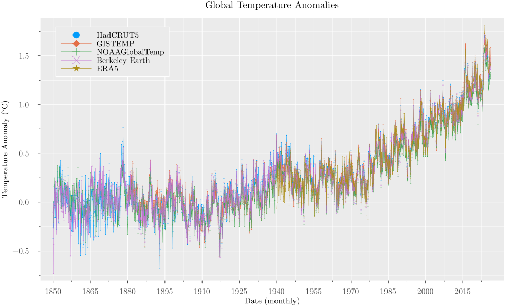

Zoom into Recent Trends

The plot shows accelerating warming and recent exceedance of the 1.5°C threshold in monthly anomalies. Zoom into the recent 30-year period to better visualize trends and ENSO variability:

compiled_zoomed = compiled_data[compiled_data.Date .>= Date(1995, 1, 1), :]

# 30-year plot
p_zoomed = plot(
    compiled_zoomed.Date, compiled_zoomed[!, series_specs[1][2]],
    title="Global Temperature Anomalies (Last 30 Years)", label=series_specs[1][1],
    xlabel="Date (monthly)", ylabel="Temperature Anomaly (°C)",
    linewidth=0.5, markershape=series_specs[1][3], markersize=1,
)

for (label, col, marker) in series_specs[2:end]
    plot!(compiled_zoomed.Date, compiled_zoomed[!, col], label=label, linewidth=0.5, markershape=marker, markersize=1)
end

plot!(legend=:topleft, xticks=(compiled_zoomed.Date[1:60:end], Dates.format.(compiled_zoomed.Date[1:60:end], "Y")))
display(p_zoomed)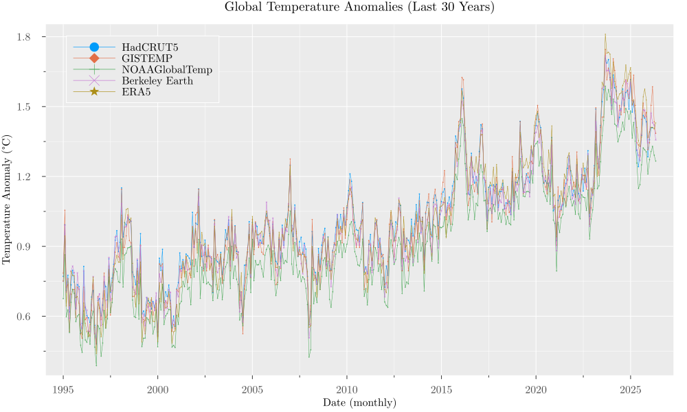

Global Temperature Anomalies (Last 30 Years)

Adding ENSO Phases

Overlay El Niño and La Niña events on the 30-year plot to distinguish ENSO variability from underlying warming. Classify ONI values into three categories: El Niño (≥+0.5°C, red shading), La Niña (≤−0.5°C, blue shading), and Neutral (between).

# Classify ONI into El Niño, La Niña, and Neutral phases
ONI_Anom = compiled_zoomed.ONI_Anomaly[.!ismissing.(compiled_zoomed.ONI_Anomaly)]
indicator = zeros(Int, length(ONI_Anom))
for i in 1:length(ONI_Anom)
    if ONI_Anom[i] >= 0.5
        indicator[i] = 1  # El Niño
    elseif ONI_Anom[i] <= -0.5
        indicator[i] = -1  # La Niña
    end
end

# Add shaded regions for ENSO phases to the zoomed plot
p_oni = copy(p_zoomed)
i = 1
while i <= length(indicator)
    if indicator[i] in (-1, 1)
        start_idx = i
        while i <= length(indicator) && indicator[i] == indicator[start_idx]
            i += 1
        end
        stop_idx = i - 1
        if stop_idx - start_idx >= 3  # Minimum duration filter
            color = indicator[start_idx] == 1 ? :red : :blue
            vspan!(p_oni, [compiled_zoomed.Date[start_idx], compiled_zoomed.Date[stop_idx]], color=color, alpha=0.1, label="")
        end
    else
        i += 1
    end
end
display(p_oni)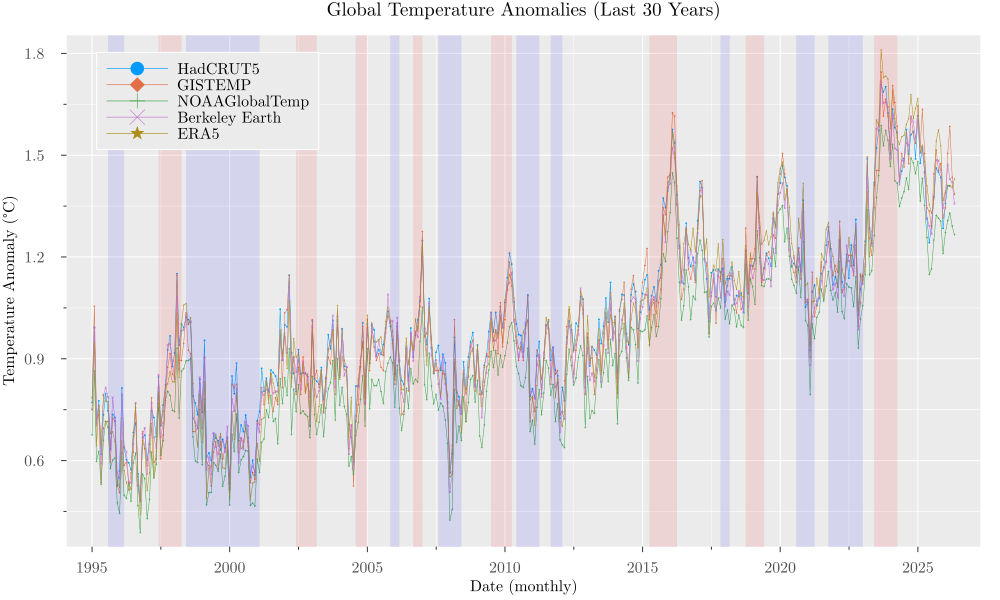

Global Temperature Anomalies with ENSO Phases

Conclusions

This paper provides a reproducible workflow for harmonising major global temperature anomaly datasets to a common 1850-1900 baseline and unified structure. The resulting dataset supports transparent cross-product comparison and consistent downstream analysis.

By combining harmonised anomaly series with ONI-based ENSO annotations, the framework separates short-term variability from the long-term warming signal. The approach is designed for reuse in climate services and policy-facing analysis, including tracking progress against Paris Agreement-related temperature targets. All code and processed datasets are openly published, supporting open-science practices and enabling independent verification and reuse across the research community. The annotated multi-dataset figures are designed for clear visual communication of temperature trends to both scientific and broader audiences.

References

Barth, Alexander. 2024. “NCDatasets.jl: A Julia Package for Manipulating netCDF Data Sets.” Journal of Open Source Software 9 (101): 6504. https://doi.org/10.21105/joss.06504.

Bezanson, Jeff, Alan Edelman, Stefan Karpinski, and Viral B Shah. 2017. “Julia: A Fresh Approach to Numerical Computing.” SIAM Review 59 (1): 65–98. https://doi.org/10.1137/141000671.

Bouchet-Valat, Milan, and Bogumił Kamiński. 2023. “DataFrames.jl: Flexible and Fast Tabular Data in Julia.” Journal of Statistical Software 107 (4): 1–32. https://doi.org/10.18637/jss.v107.i04.

Chan, Micky Yun, and JuliaClimate contributors. 2026. CDSAPI.jl. GitHub repository. https://github.com/JuliaClimate/CDSAPI.jl.

Christ, Simon, Daniel Schwabeneder, Christopher Rackauckas, Michael Krabbe Borregaard, and Thomas Breloff. 2023. “Plots.jl – a User Extendable Plotting API for the Julia Programming Language.” Journal of Open Research Software, ahead of print. https://doi.org/10.5334/jors.431.

GISTEMP. 2020. GISS Surface Temperature Analysis (GISTEMP), version 4. https://data.giss.nasa.gov/gistemp/.

Hersbach, H., B. Bell, P. Berrisford, et al. 2023. ERA5 Monthly Averaged Data on Single Levels from 1940 to Present. Copernicus Climate Change Service (C3S) Climate Data Store (CDS). https://doi.org/10.24381/cds.f17050d7.

Huang, Boyin, Xungang Yin, Tim Boyer, et al. 2025a. “Extended Reconstructed Sea Surface Temperature, Version 6 (ERSSTv6). Part i: An Artificial Neural Network Approach.” Journal of Climate (Boston MA, USA) 38 (4): 1105–21. https://doi.org/10.1175/JCLI-D-23-0707.1.

Huang, Boyin, Xungang Yin, Tim Boyer, et al. 2025b. “Extended Reconstructed Sea Surface Temperature, Version 6 (ERSSTv6). Part II: Upgrades on Quality Control and Large-Scale Filter.” Journal of Climate (Boston MA, USA) 38 (4): 1123–36. https://doi.org/10.1175/JCLI-D-24-0185.1.

Huang, Boyin, Xungang Yin, Matthew J. Menne, Russell S. Vose, and Huai-Min Zhang. 2024. NOAA Global Surface Temperature Dataset (NOAAGlobalTemp). NOAA National Centers for Environmental Information. https://doi.org/10.25921/rzxg-p717.

JuliaWeb contributors. 2026. HTTP.jl. GitHub repository. https://github.com/JuliaWeb/HTTP.jl.

Morice, Colin P, John J Kennedy, Nick A Rayner, et al. 2021. “An Updated Assessment of Near-Surface Temperature Change from 1850: The HadCRUT5 Data Set.” Journal of Geophysical Research: Atmospheres 126 (3): e2019JD032361.

NOAA National Centers for Environmental Information. 2026. Oceanic Nino Index (ONI). NOAA Climate Monitoring. https://www.ncei.noaa.gov/access/monitoring/enso/.

Quinn, Jacob, and JuliaData contributors. 2026. CSV.jl. GitHub repository. https://github.com/JuliaData/CSV.jl.

Rohde, Robert A, and Zeke Hausfather. 2020. “The Berkeley Earth Land/Ocean Temperature Record.” Earth System Science Data 12 (4): 3469–79. https://doi.org/10.5194/essd-12-3469-2020.

Citation

If you use any of the data or code in this notebook, please cite the original datasets and this notebook as follows:

Vera-Valdés, J.E. (2026). “Global Temperature Anomalies in Practice”. EarthArXiv (13310) DOI: 10.31223/X56N3Z.

@article{vera-valdesGlobalTemperatureAnomalies,
    title = {Global Temperature Anomalies in Practice},
    author = {Vera-Valdés, J Eduardo},
    year = {2026},
    journal = {EarthArXiv},
    doi = {10.31223/X56N3Z},
    url = {https://doi.org/10.31223/X56N3Z}
}

Footnotes

Note: baseline definitions may change; always check current provider documentation.↩︎
https://data.giss.nasa.gov/gistemp/faq/#q102a↩︎
The ERA5 pre-industrial offset (currently 0.88) is obtained from the ERA5 documentation.↩︎