data("AirPassengers")  #Load the data
AP = AirPassengers     #Rename it for easier access

plot(AP)   #Plot the original data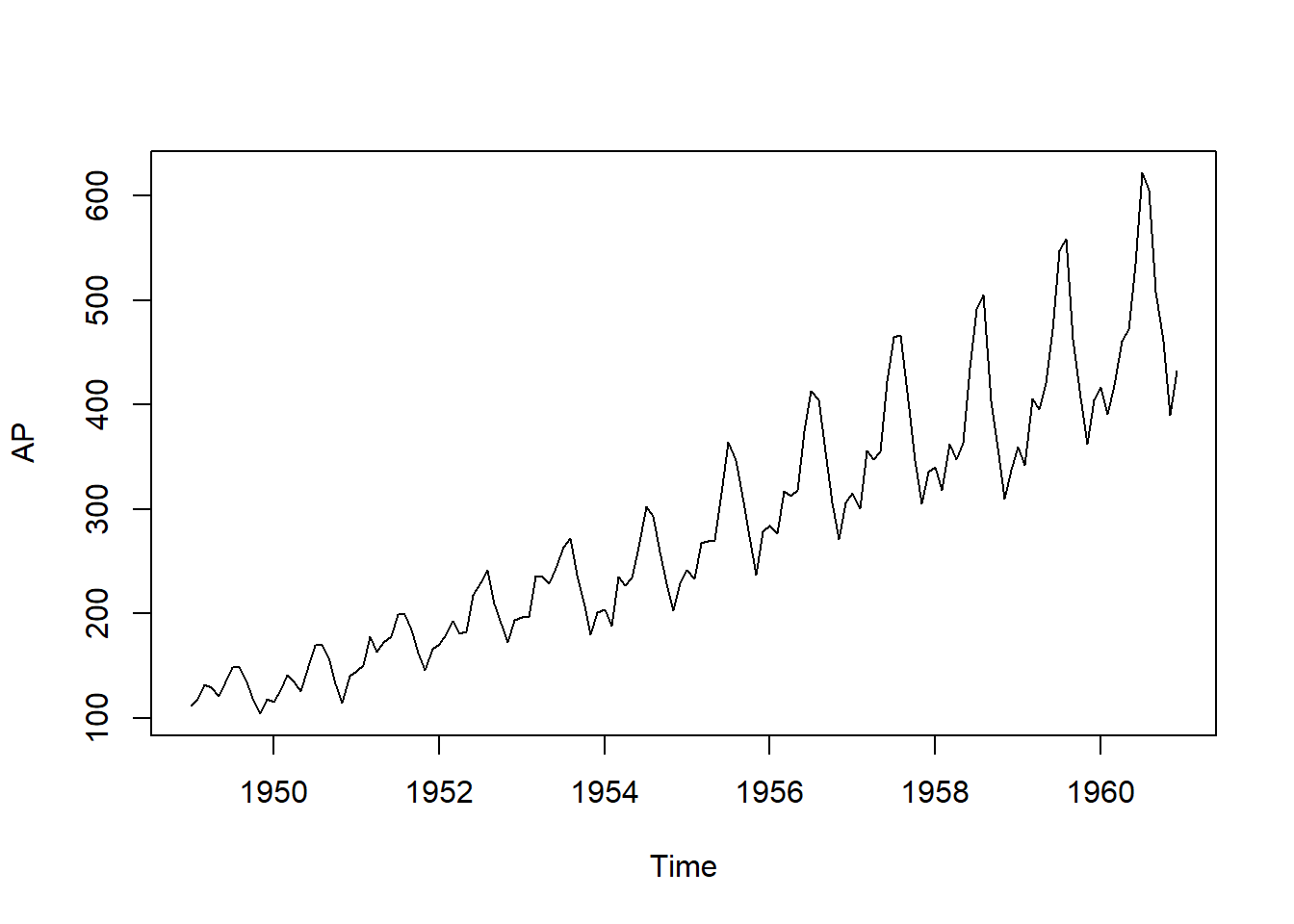
Time Series
In this self-study you are going to learn about decomposition models for time series and the exponential smoothing and Holt-Winters models. These models are widely used in practice as alternatives to the ARIMA model. Your task is to read the material and complete the exercises listed in the document.
The classical decomposition model consists of three components: trend (\(X_t\)), seasonal (\(S_t\)), and random (\(Z_t\)). The idea is to separate the time series into each of these components to analyse them separately.
There are two types of decomposition: additive and multiplicative. As the name suggests, they differ in the way the components are combined.
The most common decomposition is the additive decomposition, which is given by \[X_t = T_t + S_t + R_t.\]
Alternatively, the multiplicative decomposition is given by \[X_t = T_t \times S_t \times R_t.\]
The main difference between the two decompositions is the way the seasonal component is combined with the trend and random components. The additive decomposition is more appropriate when the seasonal component is constant over time, while the multiplicative decomposition is more appropriate when the seasonal component varies with the level of the time series. Before getting into details of how the components are estimated, let’s see an example of each decomposition.
We use the AirPassengers dataset to illustrate the decomposition models. The dataset is included with base R and it contains the monthly number of international airline passengers from 1949 to 1960. This is a classic dataset used to illustrate time series analysis.
data("AirPassengers") #Load the data
AP = AirPassengers #Rename it for easier access
plot(AP) #Plot the original data
From the plot, we can see that the seasonal component is increasing over time. That is, the ups and downs of the time series are getting larger as the level of the time series increases. This suggests that the multiplicative decomposition is more appropriate for this dataset.
The decomposition can be done using the decompose() function in R. The function requires the time series and the type of decomposition as arguments. The function returns a list with the components, which we can plot directly.
AP.deca = decompose(AP,type="additive")  #Decompose with additive model
plot(AP.deca) #Plot the decomposed additive model
Decompose the AirPassengers dataset using the multiplicative model by changing the type and plot the results.
# Your code hereWhat do you observe from the decomposition? Compare the results of the additive and multiplicative models.
The trend component is estimated by removing the seasonal and random components from the original time series. The trend is the long-term movement of the time series. It can be increasing, decreasing, or constant over time. The trend is estimated by aggregation, smoothing the time series using a moving average, or a regression model.
The simplest way to estimate the trend is by aggregating the time series in a cycle and thus smoothing it. The period of aggregation depends on the frequency of the time series. For example, if the time series is monthly, the aggregation is done over a year.
In R, the aggregate() function is used for this purpose. The function requires the time series as an argument and returns the aggregated time series.
AP.agg = aggregate(AP) #AggregatingWe can plot the aggregated time series to see the trend component.
plot(AP,ylab="")
points(1949.5:1960.5,AP.agg/12,type="o",col=4)
legend(1949,630,c("Original series","Aggregated data"),col=c(1,4),pch = c(NA,1),lty=1)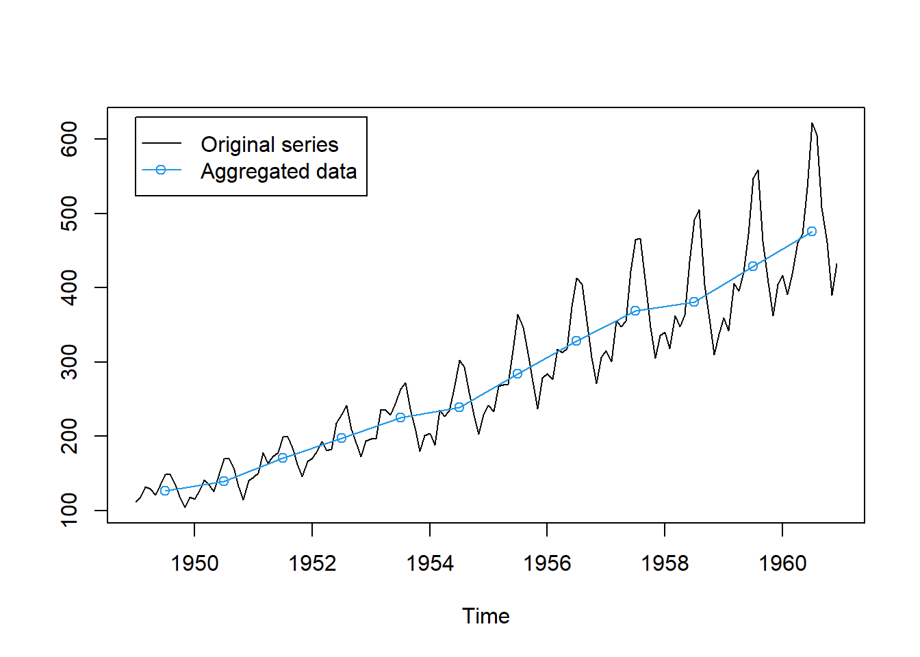
Note that we have divided the aggregated data by 12 to get the average monthly value.
The trend is smooth and captures the long-term movement of the time series. Nonetheless, aggregation discards a lot of information from the original time series. We obtain only one observation per year.
A more sophisticated way to estimate the trend component is by using a moving average. The core idea is to, instead of aggregating the time series per cycle and obtain a single observation, we can smooth the time series by averaging the observations in a window. In this sense, the moving average is a simple way to estimate the trend component, but it is more flexible than aggregation.
Note that the function decompose() in R uses a moving average to estimate the trend component. We can recover the trend component by selecting the trend component from the decomposed model using the $ operator.
The line below reports the trend component of the decomposed additive model.
AP.deca$trend Jan Feb Mar Apr May Jun Jul Aug
1949 NA NA NA NA NA NA 126.7917 127.2500
1950 131.2500 133.0833 134.9167 136.4167 137.4167 138.7500 140.9167 143.1667
1951 157.1250 159.5417 161.8333 164.1250 166.6667 169.0833 171.2500 173.5833
1952 183.1250 186.2083 189.0417 191.2917 193.5833 195.8333 198.0417 199.7500
1953 215.8333 218.5000 220.9167 222.9167 224.0833 224.7083 225.3333 225.3333
1954 228.0000 230.4583 232.2500 233.9167 235.6250 237.7500 240.5000 243.9583
1955 261.8333 266.6667 271.1250 275.2083 278.5000 281.9583 285.7500 289.3333
1956 309.9583 314.4167 318.6250 321.7500 324.5000 327.0833 329.5417 331.8333
1957 348.2500 353.0000 357.6250 361.3750 364.5000 367.1667 369.4583 371.2083
1958 375.2500 377.9167 379.5000 380.0000 380.7083 380.9583 381.8333 383.6667
1959 402.5417 407.1667 411.8750 416.3333 420.5000 425.5000 430.7083 435.1250
1960 456.3333 461.3750 465.2083 469.3333 472.7500 475.0417 NA NA
Sep Oct Nov Dec
1949 127.9583 128.5833 129.0000 129.7500
1950 145.7083 148.4167 151.5417 154.7083
1951 175.4583 176.8333 178.0417 180.1667
1952 202.2083 206.2500 210.4167 213.3750
1953 224.9583 224.5833 224.4583 225.5417
1954 247.1667 250.2500 253.5000 257.1250
1955 293.2500 297.1667 301.0000 305.4583
1956 334.4583 337.5417 340.5417 344.0833
1957 372.1667 372.4167 372.7500 373.6250
1958 386.5000 390.3333 394.7083 398.6250
1959 437.7083 440.9583 445.8333 450.6250
1960 NA NA NA NAThe window of the moving average is determined by the frequency of the time series. In the example, the time series is monthly so the window is 12. The first observation of the trend component is the average of the first 12 observations, reported in the middle of the window. Hence, note that we do not have a trend component for the first and last 6 observations. In this sense, moving average is a method that losses less information than aggregation.
Plot the trend component of the decomposed multiplicative model in a similar plot as the aggregated data above.
# Your code hereAnother way to estimate the trend component is by using a linear regression model. The linear model is given by \[X_t = \beta_0 + \beta_1 t + Z_t,\] where \(t\) is the time index and \(Z_t\) is the random component. The coefficients \(\beta_0\) and \(\beta_1\) are estimated by minimizing the sum of squared residuals.
To estimate the trend, first we generate the time index.
time = ts(1:144,start = c(1949,1),end = c(1960,12),frequency = 12)Note that we have used the ts() function to create a time series object. The start and end arguments are used to specify the start and end of the time series, respectively. The frequency argument is used to specify the frequency of the time series, which is 12 in this case.
Estimate the trend component of the AirPassengers dataset using a linear regression model with the time series as regressor. Plot the original data and the estimated trend component in a similar plot as the aggregated data above.
# Your code hereAbove we consider the simplest linear model to estimate the trend component. However, the trend component can be estimated using more complex models. For example, we can include a quadratic term in the model, or a general polynomial.
Estimate the trend component of the AirPassengers dataset using a quadratic regression model with the time series as regressor. Plot the original data and the estimated trend component in a similar plot as the aggregated data above.
# Your code hereThe seasonal component is estimated by removing the trend and random components from the original time series. The seasonal component is the short-term movement of the time series. It is the ups and downs of the time series that repeat over time.
The method to estimate the seasonal component depends on the type of decomposition. In the additive decomposition, the seasonal component is estimated by subtracting the trend from the original time series. In the multiplicative decomposition, the seasonal component is estimated by dividing the original time series by the trend.
In the code below, we plot the original time series and the seasonal component of the decomposed additive model.
ts.plot(AP,AP.deca$seasonal,col=c(1,2))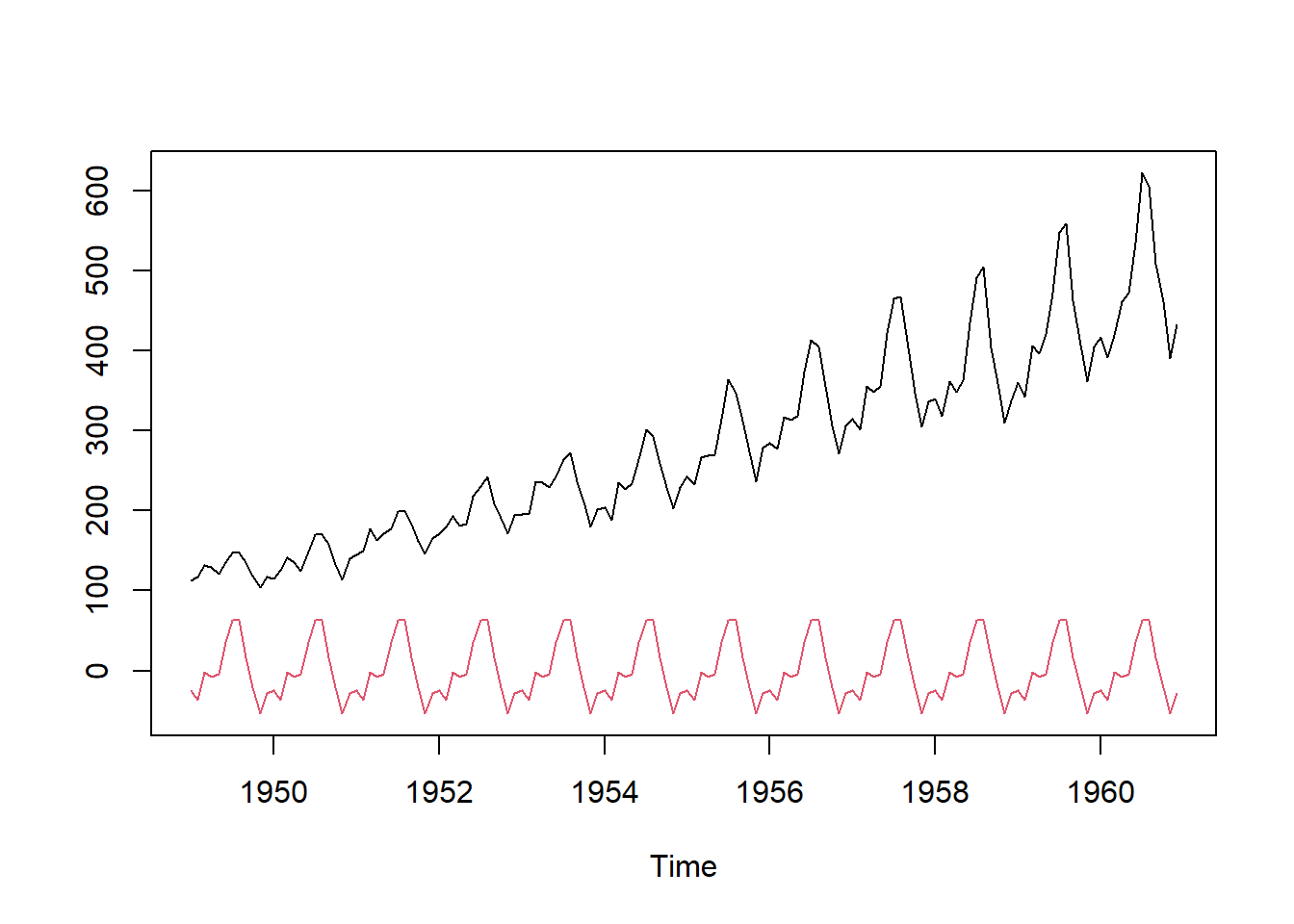
Note that the seasonal component is constant over time. This suggests that the additive decomposition is not appropriate for this dataset.
Plot the seasonal component of the decomposed multiplicative model in a similar plot as the one above.
# Your code hereThe random component is estimated by removing the trend and seasonal components from the original time series. The random component is the noise of the time series. It is the residuals of the time series after removing the trend and seasonal components.
In the code below, we plot the original time series and the random component of the decomposed additive model.
ts.plot(AP,AP.deca$random,col=c(1,2))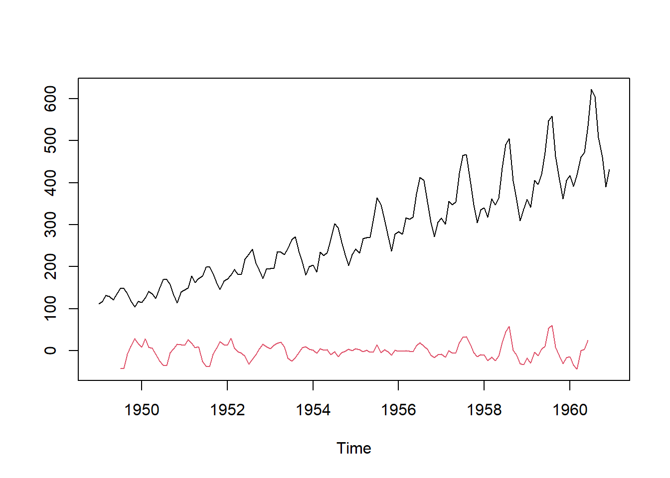
Ideally, the random component should be white noise. That is, the random component should not have any pattern. We can check this by plotting the autocorrelation function of the random component.
Plot the autocorrelation function of the random component of the decomposed additive and multiplicative models.
Hint: Use the acf() function in R to plot the autocorrelation function. You may need to omit the observations lost in the calculation of the trend, use the na.omit() function to do this.
# Your code hereWhich decomposition has a random component closer to white noise?
Exponential smoothing is a simple method to forecast time series. The method is based on the idea that present and past values of the series can be used to forecast future values. The contribution of past values decreases exponentially over time to reflect the fact that closer observations have a bigger effect.
The exponential smoothing method is given by the equation \(\begin{align*} \hat{X}_{t+1} &= \alpha X_t + \alpha(1-\alpha)X_{t-1}+\alpha(1-\alpha)^2X_{t-2}+\cdots\\ & = \alpha X_t + (1-\alpha)\hat{X}_t, \end{align*}\)
where \(\hat{X}_{t+1}\) is the forecast of the time series at time \(t+1\), \(X_t\) is the observed value at time \(t\), and \(\hat{X}_t\) is the forecast at time \(t\). The parameter \(\alpha\) is the smoothing parameter and it controls the weight of the past observations in the forecast. The parameter \(\alpha\) is between 0 and 1, and it is usually chosen by minimizing the mean squared error of the forecast.
Recursive application of the equation above gives the forecast for any time \(t+h\) as \[\hat{X}_{t+h} = \alpha X_t + (1-\alpha)\hat{X}_{t+h-1},\] which is easy to implement in practice.
The next code fits an exponential smoother to the AirPassengers dataset and plots the original data and the fitted values. The HoltWinters() function [more on this function below] is used to fit the exponential smoother. The function requires the time series as an argument and returns the fitted values. To fit the exponential smoother, we set the parameters gamma and beta to FALSE, which removes the seasonal and trend components from the model.
fit.expsm = HoltWinters(AP,gamma=F,beta=F)  #Fit the exponential smoother
ts.plot(fit.expsm$fitted,AP,col=c(1,2))     #Plot the original data and the fitted with the exponential smoother
The fitted values are very close to the original data. The exponential smoother is a simple method, but it is very effective in practice, particularly to forecast time series.
The predict() function is used to forecast future values. The function requires the fitted model and the number of periods ahead to forecast. In the example below, we predict 2 years ahead, so 24 observations. The prediction.interval argument is used to include the confidence interval in the forecast.
forecast.expsm = predict(fit.expsm,n.ahead=2*12,prediction.interval = TRUE)   #Forecasts using the exponential smoother

ts.plot(AP,forecast.expsm,lty=c(1,2,3,3),col=c(1,4,2,2))  #Plotting the original data and the forecasts with confidence interval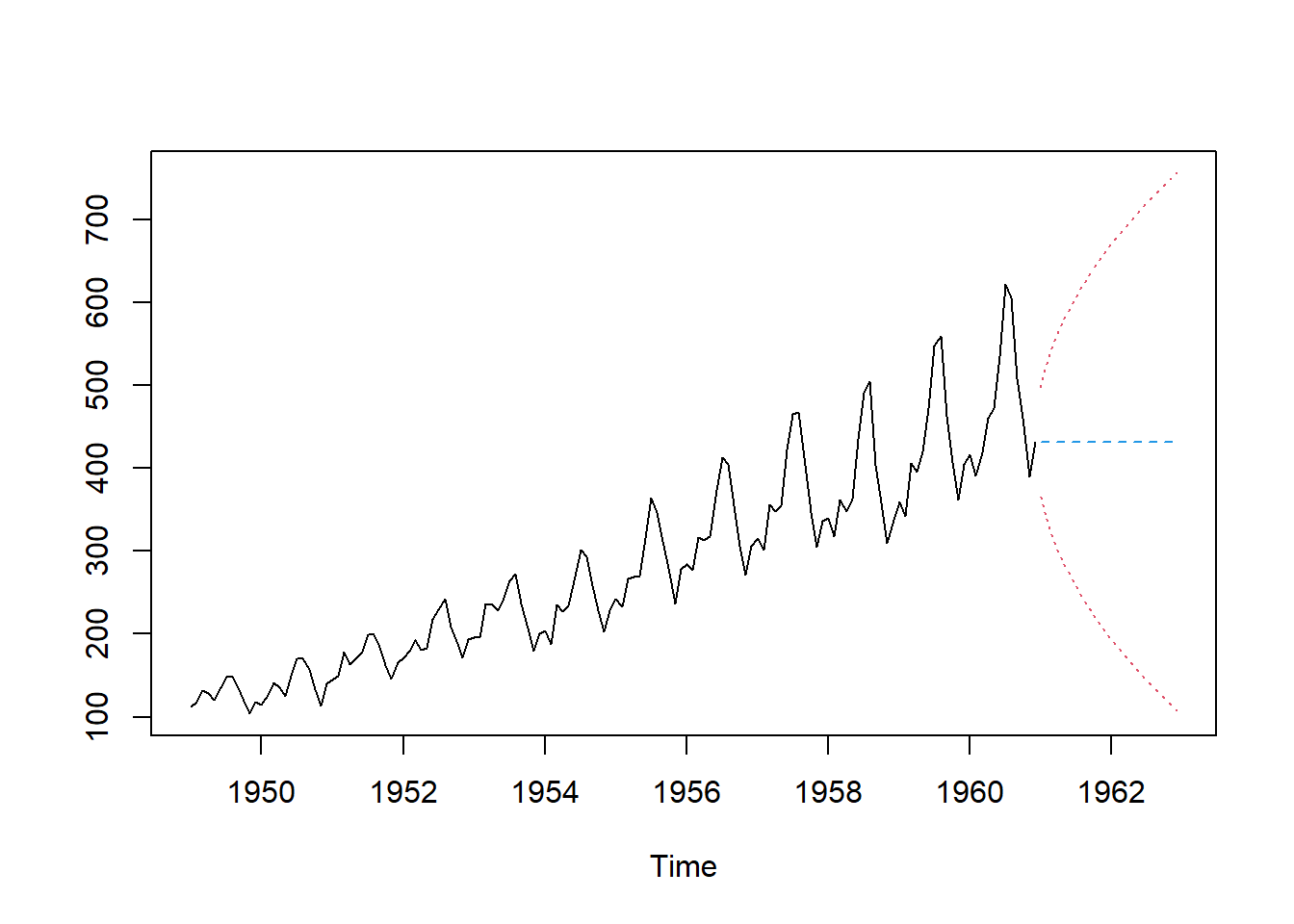
The plot shows the original data and the forecasted values. The confidence interval is also included in the plot. Note that the forecasted values are flat, which is a limitation of the exponential smoother. The method is not able to capture the trend and seasonal components of the time series. To overcome this limitation, we can use the Holt-Winters model.
The Holt-Winters model is an extension of the exponential smoother that includes the trend and seasonal components. The model is given by the equations
\(\begin{align*} \hat{X}_{t+1} &= l_t + b_t + s_{t-m+1},\\ l_t &= \alpha X_t + (1-\alpha)(l_{t-1}+b_{t-1}),\\ b_t &= \beta(l_t-l_{t-1})+(1-\beta)b_{t-1},\\ s_t &= \gamma(X_t-l_{t-1}-b_{t-1})+(1-\gamma)s_{t-m}, \end{align*}\)
where \(\hat{X}_{t+1}\) is the forecast of the time series at time \(t+1\), \(l_t\) is the level of the time series at time \(t\), \(b_t\) is the trend of the time series at time \(t\), \(s_t\) is the seasonal component of the time series at time \(t\), and \(m\) is the frequency of the time series. The parameters \(\alpha\), \(\beta\), and \(\gamma\) are the smoothing parameters of the level, trend, and seasonal components, respectively. The parameters are between 0 and 1, and they are usually chosen by minimizing the mean squared error of the forecast.
Note that the Holt-Winters model is a generalization of the exponential smoother. When the parameters \(\beta\) and \(\gamma\) are set to 0, the Holt-Winters model reduces to the exponential smoother. This is what we did in the previous section.
As used before, the HoltWinters() function is used to fit the Holt-Winters model.
Fit the Holt-Winters model to the AirPassengers dataset and plot the original data and the fitted values.
# Your code hereForecast future values of the AirPassengers dataset using the Holt-Winters model and plot the original data and the forecasted values. Include the confidence interval in the forecast.
# Your code hereWhat do you observe from the forecast? Compare the results of the exponential smoother and Holt-Winters model.
In this exercise, you are going to apply the decomposition models, exponential smoother, and Holt-Winters model to the Temperature dataset. The dataset contains the monthly Northern Hemisphere temperature anomalies from 1850. The dataset can be directly downloaded from the HadCRUT4 database. The code below downloads the data and plots the raw data.
url1 = "https://www.metoffice.gov.uk/hadobs/hadcrut4/data/current/time_series/HadCRUT.4.6.0.0.monthly_nh.txt" #Web addres of temperature data from the HadCRUT4 database

temporal = read.table(url1,sep="") #Getting the data from the url
tempn = ts(temporal[,2],start = c(1850,1), frequency = 12) #Define as time series

ts.plot(tempn) #Plotting the raw data
Aggregate the temperature data to obtain a yearly series and plot it. Can you see a trend? Comment.
# Your code hereDecompose the original (monthly) temperature data using an additive model. Plot the trend of the decomposed model and the autocorrelation function of the random component. For the ACF of the random component you will need to use the na.omit() function. Does the additive model fits the data? Comment.
# Your code hereRepeat the previous exercise using the multiplicative model.
# Your code hereEstimate the Holt-Winters model (allow for trend and seasonal components and use an additive model). Forecast 10 years of temperature data. Plot the original data and the forecast, including confidence bands. Comment.
# Your code hereIn this self-study, you have learned about decomposition models for time series and the exponential smoothing and Holt-Winters models. You have applied these models to the AirPassengers dataset and the Temperature dataset. You have learned how to decompose a time series into trend, seasonal, and random components, and how to estimate the trend, seasonal, and random components. You have also learned how to estimate the exponential smoother and Holt-Winters model, and how to forecast future values of a time series.